About
When you create a pivot table in Excel, it manipulate the data as number and when you ask to pivot a table with string value, even if you set the function to max, you will get number.
Articles Related
Solution
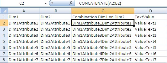
- Create a combination column and set a formula to concatenate all dimension columns values
Example with two columns : =CONCATENATE(A2;B2)
You will end up with a table as this one :
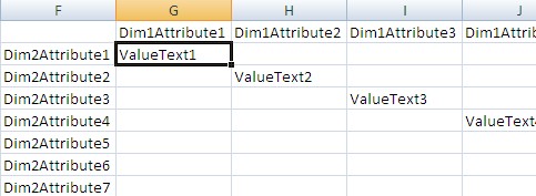
- Create the axis of the pivot table and add in the first intersection this kind of formula :
VLOOKUP(CONCATENATE(G$1;$F2);$C$2:$D$8;2;FALSE)
The V in VLOOKUP stands for vertical.
VLOOKUP :
- search the value CONCATENATE(G1;F2) which is the value of the pivot axis
- in the left column of the table C2:D8 : the combination column
- return the value of the 2 column : The column with the value
- FALSE indicate that you want and exact match. If no match is found, the value #N/A is returned. To avoid it, see the section support
- Drag the column to fill the pivot table and you obtain a pivot table for character data :
The primary key column (the combination column) must be in ascending order
Support
#N/A
To manage the #N/A, you can use the IF and ISNA function and you ends up with this formula.
=IF(ISNA(VLOOKUP(CONCATENATE(G$1;$F2);$C$2:$D$8;2;FALSE)); "";VLOOKUP(CONCATENATE(G$1;$F2);$C$2:$D$8;2;FALSE))