About
Principal Component Analysis (PCA) is a feature extraction method that use orthogonal linear projections to capture the underlying variance of the data.
By far, the most famous dimension reduction approach is principal component regression. (PCR).
PCA can be viewed as a special scoring method under the SVD algorithm. It produces projections that are scaled with the data variance. Projections of this type are sometimes preferable in feature extraction to the standard non-scaled SVD projections.
The PCR idea is to summarize the features by the principle components, which are the combinations with the highest variance.
Articles Related
Principal component
The principal components of a collection of points is the direction of a line that best fits the data while being orthogonal to the first vectors. The fit process minimizes the average squared distance from the points to the best line.
PCA can be thought of as fitting a p-dimensional ellipsoid to the data, where each axis of the ellipsoid represents a principal component. If some axis of the ellipsoid is small, then the variance along that axis is also small.
In dimensionality reduction, the goal is to retain as much of the variance in the dataset as possible. The more along the axis, the better,
Assumption
When PCR compute the principle components is not looking at the response but only at the predictors (by looking for a linear combination of the predictors that has the highest variance). It makes the assumption that the linear combination of the predictors that has the highest variance is associated with the response.
When choosing the principal component, we assume that the regression plane varies along the line and doesn't vary in the other orthogonal direction. By choosing one component and not the other, we're ignoring the second direction.
PCR looks in the direction of variation of the predictors to find the places where the responses is most likely to vary.
With principal components regression, the new transformed variables (the principal components) are calculated in a totally unsupervised way:
- the response Y is not used to help determine the principal component directions).
- the response does not supervise the identification of the principal components.
- PCR just looks at the x variables
We're just going to cross our fingers that the directions on which the x variables really vary a lot are the same directions in which the variables are correlated with the response y.
There is no guarantee that the directions that best explain the predictors will also be the best directions to use for predicting the response.
To perform an PCA analyse on a supervised way, we can instead perform partial least squares.
Steps
Getting the principal components
Getting the principal components of the data matrix x.
Procedure:
- The first principle component is just the normalized linear combination of the variables that has the highest variance.
- The second principal component has largest variance, subject to being uncorrelated with the first.
- And so on.
The principal components produces a linear combinations or dimensions of the data that are really high in variance and that are uncorrelated.
Example
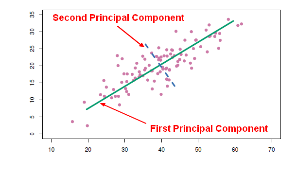
- The direction in which the data varies the most actually falls along the green line. This is the direction with the most variation in the data, this is why it's the first principal component (direction). The sum of square distances is the smallest possible.
- What's the direction along which the data varies the most out of all directions that are uncorrelated with the first direction? That's this blue dashed line. That's the second principle component in this data.
Principal Component Plot
A plot of the principle components against the variable helps to understand them better.
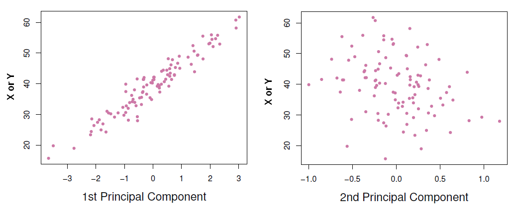
As the first principle component is highly correlated with all variables, it means that it summarizes the data very well. Then instead of using the variables X or Y to make prediction, we can use just the first principle component.
When two variables are really correlated with each other, one new variable (ie the first principle component) can really summarize both of those two variables very well.
Fitting the models with the principal components
- perform least squares regression using those principal components as predictors.
Choosing M, the number of principal component (or directions)
When more and more components are used in the regression model, the bias will decrease (because we fit more and more complex model) but the variance will then increase.
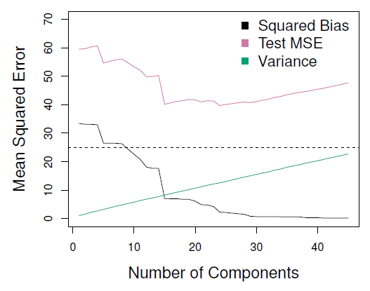
where:
- MSE has a U shape and is smallest for a model with around 18 principal components.
Cross validation was chosen in order to choose the number of principal component directions.
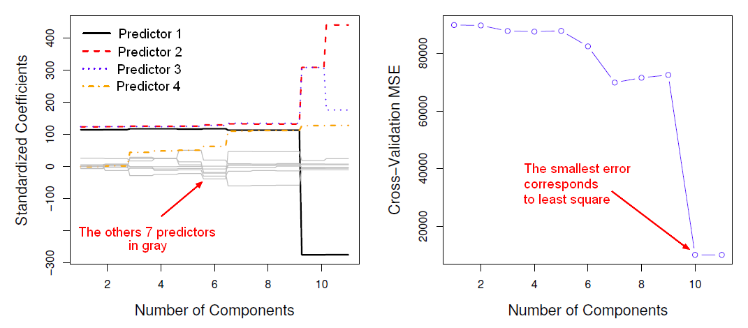
where:
- With 11 components, we got the full least squares model because when m equals p this is regular least squares on the original data.
- The cross validated mean squared error is an estimate of the test error.
In the below graphic, the mean square error is the smallest for 10 or 11 components which corresponds to least squares. Then Principal components regression doesn't give any gains over just plain least squares. Doing least squares on the original data is the best option.