About
Naive Bayes (NB) is a simple supervised function and is special form of discriminant analysis.
It's a generative model and therefore returns probabilities.
It's the opposite classification strategy of one Rule. All attributes contributes equally and independently to the decision.
Naive Bayes makes predictions using Bayes' Theorem, which derives the probability of a prediction from the underlying evidence, as observed in the data.
Naive Bayes works surprisingly well even if independence assumption is clearly violated because classification doesn’t need accurate probability estimates so long as the greatest probability is assigned to the correct class.
Naive Bayes works also on text categorization.
NB affords fast model building and scoring and can be used for both binary and multi-class classification problems.
The naive Bayes classifier is very useful in high-dimensional problems because multivariate methods like QDA and even LDA will break down.
Articles Related
Advantages / Disadvantages
Naives Bayes is a stable algorithm. A small change in the the training data will not make a big change in the model.
Assumptions
The fundamental Naive Bayes assumption is that each attribute makes an:
contribution to the outcome.
Independent
All features are independent given the target Y.
The Naive Bayes assumption say that the probabilities of the different event (ie predictors attributes) are completely independent given the class value. (i.e., knowing the value of one attribute says nothing about the value of another if the class is known)
Independence assumption is never correct but often works well in practice
The attributes must be independent otherwise they will get to much influence on the accuracy. If an attribute are dependent with the target, it's the same that to determine the accuracy of only this attribute.
You can model the dependency of an attribute by copying hem n times. Continuing to make copies of an attribute gives it an increasingly stronger contribution to the decision, until in the extreme the other attributes have no influence at all.
Equal
The event (ie predictors attributes) are equally important a priori.
If the accuracy remains exactly the same when an attribute is removed, it seems that this attribute is irrelevant to the outcome of the class (target).
Description
Formula
The Naive Bayes algorithm is based on conditional probabilities. It uses Bayes' Theorem, a formula that calculates a probability by counting the frequency of values and combinations of values in the historical data.
Bayes' Theorem finds the probability of an event occurring given the probability of another event that has already occurred.
Bayes' theorem: Probability of event A given evidence B
<math> \text{Prob(A given B)} = \frac{\displaystyle \text{Prob(A and B)}}{\displaystyle \text{Prob(A)}} </math>
where:
- A represents the dependent event: A target attribute
- and B represents the prior event: A predictors attribute
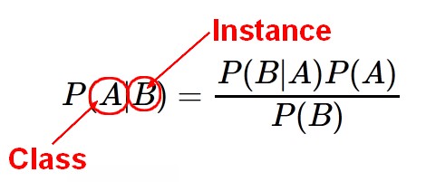
- P(A) is a priori probability of A (The prior probability) Probability of event before evidence is seen. The evidence is an attribute value of an unknown instance.
- P(A|B) is a posteriori probability of B. Probability of event after evidence is seen. Posteriori = afterwards, after the evidence
Naive
“Naïve” assumption: Evidence splits into parts that are independent
<math> P(B|A) = \frac{\displaystyle P(A_1|B)P(A_2|B) \dots P(A_n|B)}{P(B)} </math> where:
- <math>A_1, A_2, \dots, A_n</math> are totally independent priori.
Example
Spam Filtering with Naïve Bayes on a two classes problem (spam and not spam.) Bill Howe, UW
The probability that an email is span given the email words is:
<math> \begin{array}{rrl} P(spam|words) & = & \frac{\displaystyle P(spam) . P(words|spam)}{\displaystyle P(words)} \\ & = & \frac{\displaystyle P(spam) . P(viagra, rich, \dots, friend|spam)}{\displaystyle P(viagra, rich, \dots, friend)} \\ & \propto & P(spam).P(viagra, rich, \dots, friend|spam) \\ \end{array} </math>
where:
- <math>\propto</math> is the proportion symbol
Using the Chain rule:
- One Time: <math>P(spam|words) \propto P(spam).P(viagra|spam).P(rich, \dots, friend|spam, viagra)</math>
- Two Time: <math>P(spam|words) \propto P(spam).P(viagra|spam).P(rich|spam, viagra)*P(\dots, friend|spam, viagra, rich)</math>
Saying that the word events are completely independent permit to simplify the above formula to a sequential use of the Bayes' formula such as:
<math>P(spam|words) \propto P(viagra|spam)*P(rich|spam)*\dots*P(friend|spam)</math>
Discriminant Function
This is the discriminant function for the kth class for naive Bayes. You compute one of these for each of the classes, then you classify it.
<MATH> \delta_k(x) \approx log \left [ \pi_k \prod^p_{j=1} f_{kj}(x_j) \right ] = -\frac{1}{2} \sum^p_{j=1}\frac{(x_j - \mu_{kj})^2}{\sigma^2_{kj}} + log(\pi_k) </MATH>
There's:
- a determinant term which is a contribution of the feature from the mean for the class scaled by the variance, <math>\frac{\displaystyle (x_j - \mu_{kj})^2}{\displaystyle \sigma^2_{kj}}</math>
- a prior term <math>log(\pi_k)</math>
NB can be used for mixed feature vectors (qualitative and quantitative).
- For the quantitative ones, we use the Gaussian.
- For the qualitative ones, we replace the density function <math>f_kj(x_j)</math> with probability mass function (histogram) over discrete categories.
And even though it has strong assumptions, it often produces good classification results.
Example
Weather Data Set
With the Weather Data Set:
P(A and B)
| Outlook | Temperature | Humidity | Wind | ||||||||||||||||
|---|---|---|---|---|---|---|---|---|---|---|---|---|---|---|---|---|---|---|---|
| Yes | No | P(Yes) | P(No) | Yes | No | P(Yes) | P(No) | Yes | No | P(Yes) | P(No) | Yes | No | P(Yes) | P(No) | ||||
| Sunny | 2 | 3 | 2/9 | 3/5 | Hot | 2 | 2 | 2/9 | 2/5 | High | 3 | 4 | 3/9 | 4/5 | False | 6 | 2 | 6/9 | 2/5 |
| Overcast | 4 | 0 | 4/9 | 0/5 | Mild | 4 | 2 | 4/9 | 2/5 | Normal | 6 | 1 | 6/9 | 1/5 | True | 3 | 3 | 3/9 | 3/5 |
| Rainy | 3 | 2 | 3/9 | 2/5 | Cool | 3 | 1 | 3/9 | 1/5 | ||||||||||
| Total | 9 | 5 | 100% | 100% | Total | 9 | 5 | 100% | 100% | Total | 9 | 5 | 100% | 100% | Total | 9 | 5 | 100% | 100% |
To get rid of the zero (Zero Frequency Problem, 0*n = 0), add one to all the kinds.
P(A)
| Play | P(Yes) / P(No) | |
|---|---|---|
| Yes | 9 | 9/14 |
| No | 5 | 5/14 |
| Total | 14 | 100% |
P(A and B)
What is the probability of Yes and No on a new day with the following characteristics (evidence ?): Rainy, Cool, High, True.
<math> \begin{array}{rrr} P(Yes|New Day) & = & \frac{P(Rainy Outlook |Yes).P(Cool Temperature |Yes).P(High Humidity|Yes).P(With Wind|Yes).P(Play|Yes)}{P(New Day) } \end{array} </math>
P(New Day) is unknown but it doesn't matter because the same equation can be done for No and it sums up to one with the Yes probability:
<math> P(yes|New Day)+P(no|New Day)=1 </math>
The proportional probabilty are then:
<math> \begin{array}{rrrrr} P(Yes|New Day) & \propto & \frac{3}{9} . \frac{3}{9} . \frac{3}{9} . \frac{3}{9} . \frac{9}{14} & \approx & 0.0079 \\ P(No|New Day) & \propto & \frac{2}{5} . \frac{1}{5} . \frac{4}{5} . \frac{3}{5} . \frac{5}{14} & \approx & 0.0137 \\ \end{array} </math>
This numbers can be converted into a probability by making the sum equal to 1 (normalization):
<math> \begin{array}{rrrrr} P(Yes|New Day) & = & \frac{0.0079}{0.0079+0.0137} & = & 0.36 \\ P(No|New Day) & = & \frac{0.0137}{0.0079+0.0137} & = & 0.63 \\ \end{array} </math>
The answer is then NO.
To test
To calculate the probability of A given B, the algorithm counts the number of cases where A and B occur together and divides it by the number of cases where B occurs alone.