
About
Multiple regression is a regression with multiple predictors. It extends the simple model. You can have many predictor as you want. The power of multiple regression (with multiple predictor) is to better predict a score than each simple regression for each individual predictor.
In multiple regression analysis, the null hypothesis assumes that the unstandardized regression coefficient, B, is zero.
Articles Related
(Equation | Function)
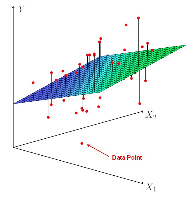
The function is called a hyperplane.
In general notation:
<MATH> \begin{array}{rrl} \hat{Y} & = & Y - e \\ & = & B_0 + B_1.{X_1} + B_2.{X_2} + \dots + B_k.{X_k} - e\\ & = & B_0 + \sum_{1}^{k}(B_k.{X_k}) - e\\ \end{array} </MATH>
where:
- <math>Y</math> is the original score
- <math>\hat{Y}</math> is the predicted score (ie the model)
- <math>e</math> is the error (residual) ie <math>Y - \hat{Y}</math>
- <math>B_0</math> is the intercept also known as the regression constant
- <math>B_k</math> is the slope also known as the regression coefficient
- <math>X_k</math> are predictor variables
- <math>k</math> is the number of predictor variables
The intercept is the point in the Y axis when X is null. And the slope tells that for each X units (1 on the X scale), Y increases of the slope value.
Regression Coefficient
Interpretation
Balanced design
The ideal scenario is when the predictors are uncorrelated (a balanced design).
- Each coefficient can be estimated and tested separately.
- Interpretations such as “a unit change in <math>X_j</math> is associated with a <math>B_ j</math> change in Y , while all the other variables stay fixed”, are possible.
But predictors are not usually uncorrelated in the data. They will tend to move together in real data.
Unbalanced design
Correlations amongst predictors cause problems:
- The variance of all coefficients tends to increase, sometimes dramatically
- Interpretations become hazardous. when <math>X_j</math> changes, everything else changes. The Regression coefficients in multiple regression must be interpreted in the context of the other variables.
We might get a particular regression coefficient on a variable just because of others characteristics of the sample.
The value of one regression coefficient is influenced by the other values on the other variables that are used as predictors in the model.
The calculation of one regression coefficient is made taking into account the other variables. You can only make cross conclusion between all variables from all regression coefficients.
�A regression coefficient �<math>B_j</math> estimates the expected change in Y per unit change in <math>X_j</math> , with all other predictors held fixed.
But predictors usually change together.
Claims of causality should be avoided because the predictors in the system are correlated. (ie One predictor doesn't cause the outcome).
Any effect of a predictor variable can be soaked up by an other because they're correlated. And on the other hand, uncorrelated variables may have somewhat complimentary effects.
Strongest predictor
The strongest predictor is given by the standardized regression coefficient.
Estimation of Standardized Coefficient
The values of the coefficients (B) are estimated such that the model yields optimal predictions by minimizing the sum of the squared residuals (RSS). This method is called the multiple least squares estimates because there's multiple predictors.
Ie A multiple regression fits a hyperplane to minimize the square distance between each point and the closest point on the plane.
Step 1
The linear matrix equation (regression model)
<math>\hat{Y} = B.X</math>
where:
- <math>\hat{Y}</math> is a [N x 1] vector representing the predicted score where N is the sample size
- <math>X</math> is the [N x k] design matrix representing the predictors variables where k is the number of predictors
- <math>B</math> is a [k x 1] vector representing the regression coefficients (<math>\beta</math> )
- the regression constant is assumed to be zero.
Step 2
Assuming that the residual are null, <math>\hat{Y} = Y</math>
<math>Y = X.B</math>
where <math>Y</math> is the raw score
Step 3
To make X square and symmetric in order to invert it in the next step
only square matrices can be inverted
, both sides of the equation are pre-multiplied by the Linear Algebra - Matrix of X.
<math>X^T.Y = X^T.X.B</math>
Step 4
To eliminate <math>X^T.X</math> , pre-multiply by the inverse, <math>(X^T.X)^{-1}</math> because <math>(X^T.X).(X^T.X)^{-1}= I</math> where I is the identity matrix
<math> \begin{array}{rrl} (X^T.X)^{-1}.(X^T.Y) & = & (X^T.X).(X^T.X)^{-1}.B \\ (X^T.X)^{-1}.(X^T.Y) & = & B \\ B & = & (X^T.X)^{-1}.(X^T.Y) \end{array} </math>
Step 5
Substitute:
- <math>(X^T.X)^{-1}</math> with “Sum Square of Deviation Score and Som of cross product” matrix
- <math>(X^T.Y)</math> with “Sum Square of Deviation Score and Som of cross product” matrix
<math> \begin{array}{rrl} B & = & (X^T.X)^{-1}.(X^T.Y) \\ & = & {S_{xx}}^{-1}.S_{xy} \\ \end{array} </math>
Confidence Interval
If the confidence intervals don't cross zero (if they don't include zero), it's an indication that they're going to be significant.
Visualisation
You can't visualize multiple regression in one graphic (scatter-plot) because they are more than one predictors. There is one way through the model R and R squared to capture it all in one scatter plot.
By saving the predicted scores, you can plot an other scatter plot with the predicted scores on the x axis vs the actual score on the y axis.
Questions
Question that can be answered from the model.
- Is at least one of the predictors <math>X_1,X_2,\dots,X_n</math> useful in predicting the response?
- Do all the predictors help to explain Y , or is only a subset of the predictors useful?
- Given a set of predictor values, what response value should we predict, and how accurate is our prediction?
Question that can be answered from alternative models..
- How well does the model fit the data?
One predictor Useful ?
To answer the question: Is at least one of the predictors <math>X_1,X_2,\dots,X_n</math> useful in predicting the response? we can use the F-statistic
We look at the drop in training error (ie the present variance explained R Squared). To quantify it in a more statistical way, we can form the f-ratio.
<MATH> F = \frac{\displaystyle \frac{(TSS-RSS)}{p}}{\displaystyle \frac{RSS}{n-(p+1)}} </MATH>
The f-statistic is:
- the drop in training error (TSS-RSS) divided by the number of parameters (p)
- divided by the mean squared residual
- ie rss divided by
- the sample size N minus the number of parameters we fit (p plus 1 for the intercept).
Under the null hypothesis (ie there's no effect of any of predictors), the f-statistic will have an f-distribution with p and n minus p minus 1 degrees of freedom.
Variables importance
What are the important variables to include in the model. See Data Mining - (Attribute|Feature) (Selection|Importance)
Variables redundant ?
We don't want to include variables that are redundant. One of them is not going to explain a significant amount of variants in the outcome when the other one is in the model. Because they're both sort of explaining the same variants.
When multiple regression coefficient remains significant these two variables are not redundant and our prediction should get better by including both of these in the model over including just one alone.