
About
A Simple Linear regression is a linear regression with only one predictor variable (X).
Correlation demonstrates the relationship between two variables whereas a simple regression provides an equation which is used to predict scores on an outcome variable (Y).
Articles Related
Linear Equation
In a standard notation:
<math>
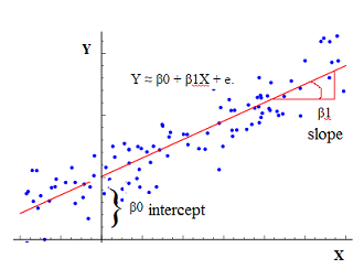
Y = m + b.X + e
</math>
or in a general notation (that introduces the idea of multiple regression):
<math>
Y = \hat{Y} + e = (B_0 + B_1.{X_1}) + e
</math>
where:
- <math>Y</math> is the original target score (as a linear function of <math>X \,(X_1)</math> )
- <math>\hat{Y}</math> is the predicted target score (ie the model)
- <math>e</math> is the error (residual) ie <math>Y - \hat{Y}</math>
- (<math>m</math> of <math>B_0</math> ) is the intercept also known as the regression constant
- (<math>b</math> of <math>B_1</math> ) is the slope also known as the regression_coefficient. Within a simple regression, the standardized regression coefficient is the same as the correlation coefficient
The intercept is the point in the Y axis when X is null. And the slope tells that for each X units (1 on the X scale), Y increases of the slope value.
The intercept and the slope are also known as coefficients or parameters.
Assumptions
The distribution of the error (residual) is normally distributed.
Estimation of the parameters
The values of the regression coefficients are estimated such that the regression model yields optimal predictions.
The regression coefficient is what we observed.
In simple regression, the standardized regression coefficient will be the same as the correlation coefficient
(Ordinary) Least Squares Method
An optimal prediction for one variable is reached:
- by minimizing the residuals (ie the predictions errors),
- ie by minimizing the overall distance between the line and each individual dot <math>\displaystyle \sum_{i=1}^{N}(Y_i - \hat{Y}_i)</math> .
- ie by minimizing the sum of the squared residuals (RSS)
This idea is called the Ordinary Least Squares estimation.
The least squares approach chooses <math>B_0</math> and <math>B_1</math> to minimize the Residual sum of Squares (RSS).
<MATH> \begin{array}{rrl} \hat{B}_1 & = & \frac { \displaystyle \sum_{i=1}^{\href{sample_size}{N}} (X_i - \href{mean}{\bar{X}})(Y_i - \href{mean}{\bar{Y}}) } { \displaystyle \sum_{i=1}^{\href{sample_size}{N}} (X_i - \href{mean}{\bar{X}})^2 } \\ \hat{B}_0 & = & \href{mean}{\bar{Y}} - \hat{B}_1 . \href{mean}{\bar{X}} \end{array} </MATH>
Formula
Unstandardized
Formula for the unstandardized coefficient
<MATH> \text{Regression Coefficient (Slope)} = \href{little_r}{r} . \frac{\href{Standard Deviation}{\text{Standard Deviation of Y}}}{\href{Standard Deviation}{\text{Standard Deviation of X}}} </MATH>
where:
- r is little r
- Standard deviation is Standard deviation
The standard deviation division is needed in order to take into account the scale and variability of X and Y.
Standardized
In the z scale, the standard deviation is 1 and the mean is zero. The Regression Coefficient becomes there:
<MATH> \begin{array}{rrl} \text{Standardized Regression Coefficient - } \beta & = & \href{little_r}{r} . \frac{\href{Standard Deviation}{\text{Standard Deviation of Y}}}{\href{Standard Deviation}{\text{Standard Deviation of X}}} \\ \beta & = & \href{little_r}{r}.\frac{1}{1} \\ \beta & = & \href{little_r}{r} \\ \end{array} </MATH>
The coefficient are standardized to be able to compare them. For instance, in a multiple regression. The unstandardized coefficient are linked to the scale of each predictor and therefore can not be compared.
Accuracy
The Accuracy can be assessed for:
- the parameters
- the overall model
Parameters
The slope of the predictor can be assess , both in terms of:
- confidence intervals
- and hypothesis test.
Standard Error
The standard error is the standard deviation calculated on the error distribution. (assuming that it's normal).
<MATH> \begin{array}{rrl} SE(\hat{B}_1)^2 & = & \frac{ \displaystyle \sigma^2}{\displaystyle \sum_{i=1}^{N}(X_i - \bar{X})^2} \\ SE(\hat{B}_0)^2 & = & \sigma^2 \left [ \frac{1}{N} + \frac{ \displaystyle \bar{X}^2 } { \displaystyle \sum_{i=1}^{N}(X_i - \bar{X})^2 } \right ] \\ \end{array} </MATH>
where
- sigma square is the noise (ie the variance of the square around the line). <math>\sigma^2 = \href{variance}{var}(\href{residual}{\epsilon})</math>
These standard errors (SE) are used to compute con�fidence intervals.
Confidence Interval
<MATH> \begin{array}{rrl} \hat{B}_1 & = & 2.SE(\hat{B}_1) \end{array} </MATH>
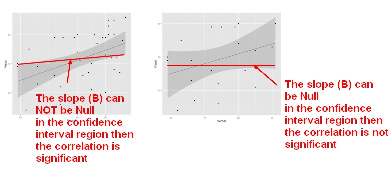
As we assume that the errors are normally distributed, there is then approximately a 95% chance that the following interval will contain the true value of <math> B_1</math> (under a scenario where we got repeated samples ie repeated training set). If we calculate 100 confidence intervals on 100 sample data set, 95% of the time, they will contain the true value.
<MATH> \begin{array}{rrl} [ \hat{B}_1 - 2.SE(\hat{B}_1) , \hat{B}_1 + 2.SE(\hat{B}_1) ] \end{array} </MATH>
Visually, if we can't get a flat regression line (Slope = 0) in confidence interval region (the shadowed one), it means that it's a significant effect.
t-statistic
Standard errors can also be used to perform a null hypothesis tests on the coefficients. It corresponds to testing:
- <math>H_0 : B_1 = 0 </math> (Expected Slope, Null Hypothesis)
- versus <math>H_A : B_1 \neq 0 </math> (Observed Slope).
To test the null hypothesis, a t-statistic is computed:
<MATH> \begin{array}{rrl} \text{t-value} & = & \frac{(\text{Observed Slope} - \text{Expected Slope})}{\href{Standard Error}{\text{What we would expect just due to chance}}} & \\ \text{t-value} & = & \frac{\href{regression coefficient#unstandardised}{\text{Observed Slope}} - 0}{\href{Standard Error}{\text{What we would expect just due to chance}}}\\ \text{t-value} & = & \frac{\href{regression coefficient#unstandardised}{\text{Unstandardised regression coefficient}}}{\href{Standard Error}{\text{Standard Error}}}\\ \text{t-value} & = & \frac{\hat{B}_1}{SE(\hat{B}_1)} \\ \end{array} </MATH>
where:
This t-statistic will have a t-distribution with n - 2 degrees of freedom, assuming <math>B_1 = 0</math> which gives us all elements to compute the p-value
The probability (p-value) is the chance of observing any value equal to <math>|t|</math> or larger. In a linear regression, when the p value is less than 0.5 we will reject the null hypothesis.
With a p-value of for instance, 10 to the minus 4, the chance of seeing this data, under the assumption that the null hypothesis (There's no effect, ie no relationship, ie the slope is null ) is less than the p-value (10 to the minus 4). In this case, it's very unlikely to have seen this data. It's possible, but very unlikely under the assumption that the predictor X has no effect on the outcome Y. The conclusion, therefore, will be that the predictor X has an effect on the outcome Y.
Model
Residual Standard Error (RSE)
<MATH> \begin{array}{rrl} \text{Residual Standard Error (RSE)} & = & \sqrt{\frac{1}{n-2}\href{rss}{\text{Residual Sum-of-Squares}}} \\ RSE & = & \sqrt{\frac{1}{n-2}\href{rss}{RSS}} \\ RSE & = & \sqrt{\frac{1}{n-2}\sum_{i=1}^{N}(Y_i -\hat{Y}_i)} \\ \end{array} </MATH>
R (Big R)
For a simple regression, R (Big R) is just the correlation coefficient, little r squared.
R-squared
R-squared or fraction of variance explained measures how closely two variables are associated.
<MATH> \begin{array}{rrl} R^2 & = & \frac{\href{tss}{TSS} - \href{rss}{RSS}}{\href{tss}{TSS}} \\ R^2 & = & 1 - \frac{\href{rss}{RSS}}{\href{tss}{TSS}} \\ \end{array} </MATH>
where:
- TSS is the error of the simplest model
- RSS is the error after optimization with the least squares method.
This statistic measures, how much was reduced the total sum of squares (TSS-RSS) relative to itself (TSS). So this is the fraction of variance explained.
In this simple linear regression, <math>R^2 = r^2</math> , where r is the correlation coefficient between X and Y.
The higher the correlation, the more that we'll explain the variance.
A value <math>R^2 = 0.51</math> means that the variance was reduced by 51%.
A <math>R^2 = 0.9 </math> indicates a fairly strong relationship between X and Y.
The domain of application is really important to have a judgement of how good an R squared is. Example of good value by domain:
- In business, financial application and some kind of physical sciences: <math>R^2 \approx 0.51</math>
- In medicine, <math>R^2 \approx 0.05</math>